Bare-bones Pandas

Pandas' syntax is often bashed for being confusing as there are multiple ways of achieving the same output, with some subtle differences. Let's look at the most common Pandas methods and compare them.

Mar 27, 2023

Pandas is a popular data manipulation library in Python, but its syntax is often criticized for being confusing. There are multiple ways to achieve the same output, and these methods may have subtle differences. In this blog post, we will examine the most common Pandas methods and compare them, so you can choose the best approach for your data manipulation needs.

A small part of Python’s Pandas library makes up the majority of data manipulation methods that a data engineer or analyst might utilise. Knowing about the most common operations and methods used will also save you time, before needing to dive deep into the documentation.

Share Modern Data Engineering

Selecting columns from a dataframe

With Pandas there are two ways of selecting columns from a dataframe and returning a series object:

Using brackets:

df['column_name']

Using dot notation

df.column_name

While dot notation is a convenient way to access columns in a Pandas dataframe, there are certain situations where it won't work as expected. Dot notation will not work when there are:

Spaces in the column name.
If the column name is the same as the name of a dataframe method or when the column name is a variable.
If the column name is stored in a variable that holds a reference to the column name, e.g. col = 'count'.

If the column name is stored in a variable, dot notation won't work and you'll need to use square brackets instead.

For example, if you have a dataframe with a column named "count", running df.count with dot notation will actually generate a reference to the method count for the dataframe, rather than returning the column. To retrieve the column data, you'll need to use square brackets, like so: df['count'].

The same applies when the column name is stored in a variable. If you have a variable col that holds a reference to the column name, like col = 'count', you'll need to use square brackets to return the column using the variable: df[col]. By being aware of these limitations, you can use the appropriate notation for accessing dataframe columns in all situations.

Checking for nulls

If there is more than one way of generating the exact same output, the methods are called aliases. The isna() and isnull() methods are aliases because they both check for any null values in the data.

Similarly, the notna() and notnull() methods are aliases that perform the opposite operation of isna() and isnull(), checking for non-null values instead. While it's good to have different methods for the same operation, using too many aliases can make your code harder to read and maintain. To keep things consistent, I prefer to stick to using only isna() and notna() whenever possible to avoid confusion.

Operators vs equivalent methods

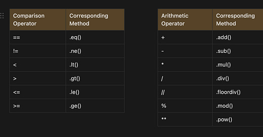
The arithmetic and comparison operators have corresponding methods that can be used to do the same thing.

Operator methods allow you to perform arithmetic operations on dataframes, but they also include parameters like axis that give you greater control over how the operation is performed. For instance, this would change what happens if we tried to divide the values within a column of a dataframe by values in another column of a series. By setting axis=’index’ within the method we would ensure the index of the dataframe aligns with the index of the series.

df = df.div(series, axis='index')

Group by and aggregations

There are a few choices of syntax for performing group by aggregations and some are less verbose than others, making it easier to read and understand, while others utilise a dictionary to map columns to aggregation methods.

With a dictionary-based approach, you can specify the desired aggregation method for each column individually, allowing you to fine-tune the analysis to your specific needs.

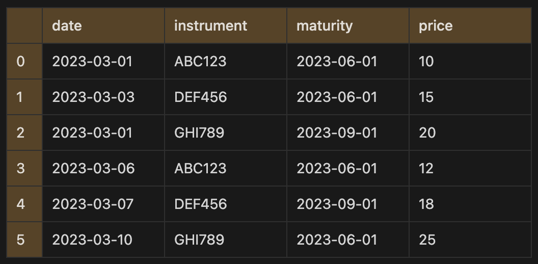
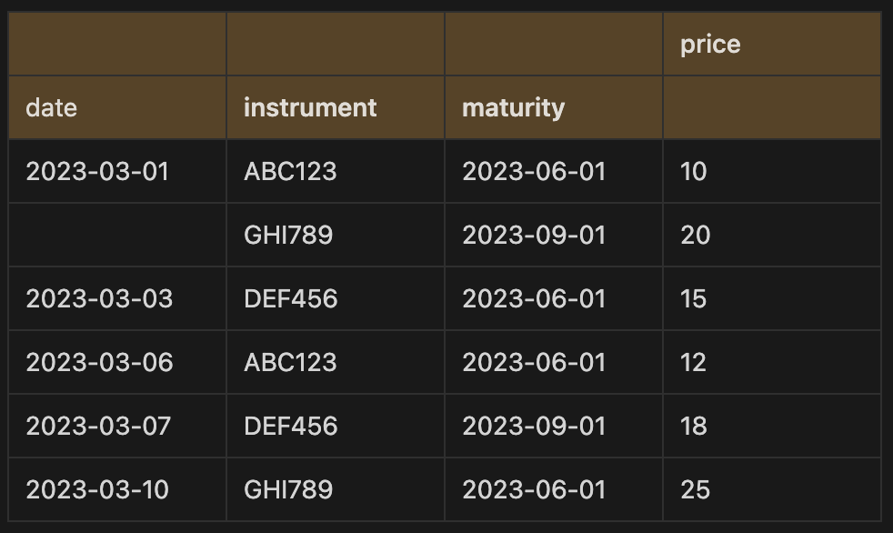
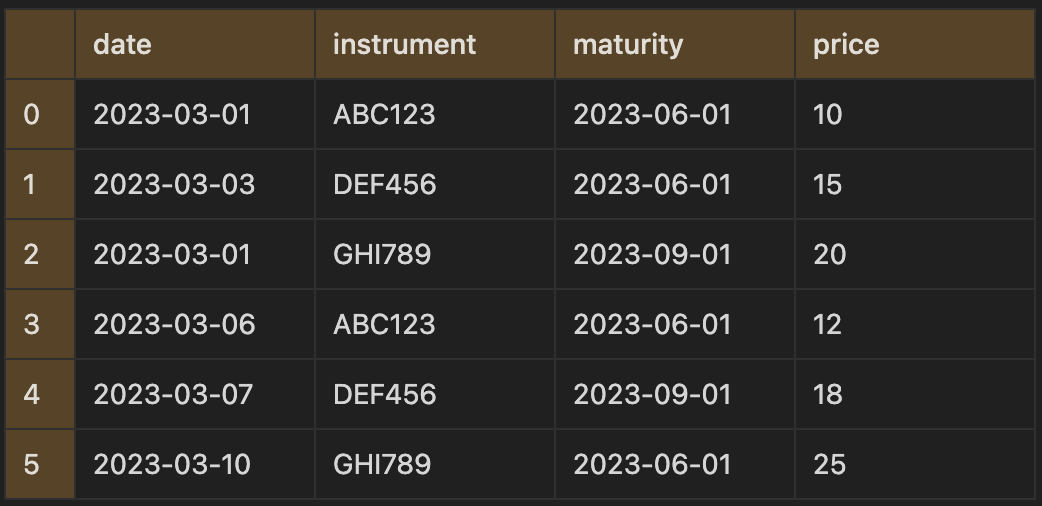
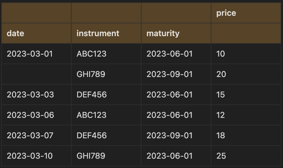
Let’s take some made up trading data for instruments with their prices. If we wanted to group by the date, instrument and maturity to sum the price per group and count the number of trades per group we could write the two following lines of code:

trades_df.groupby(["date", "instrument", "maturity"]).agg({"price": "sum"})

trades_df.groupby(['date', 'instrument', 'maturity'])['price'].agg('sum')

date instrument maturity

2023-03-01 ABC123 2023-06-01 10
GHI789 2023-09-01 20
2023-03-03 DEF456 2023-06-01 15
2023-03-06 ABC123 2023-06-01 12
2023-03-07 DEF456 2023-09-01 18
2023-03-10 GHI789 2023-06-01 25
Name: price, dtype: int64

The first one returns a dataframe, whereas the second form has the aggregating column within the brackets and returns a series object. In this instance, you could also call the aggregating method sum() and it would return the same series as in the second option:

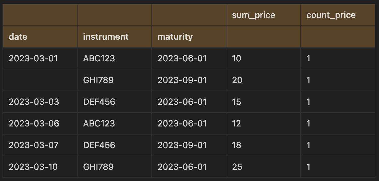
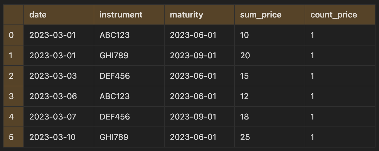
trades_df.groupby(['date', 'instrument', 'maturity'])['price'].sum()

As things become more complex, it makes sense to use Pandas NamedAgg method which accepts keyword arguments and is verbose, making it more readable when performing different aggregations on multiple columns and names columns easily. For example, if we take the trades dataset and perform the same grouping but this time count the number of trades and sum the prices, we could write:

trades_df.groupby(['date', 'instrument', 'maturity']).agg(
    sum_price = pd.NamedAgg('price', 'sum'),
    count_price = pd.NamedAgg('date', 'count')
)

In fact, the agg method knows to instantiate the many keyword arguments tuples as NamedAgg’s, meaning you can remove the pd.NamedAgg part to improve readability and maintainability of your code.

trades_df.groupby(['date', 'instrument', 'maturity']).agg(
    sum_price = ('price', 'sum'),
    count_price = ('date', 'count')
)

When you're working with time-series data, it's often useful to calculate rolling aggregates over a fixed window period. This can help you identify trends and patterns in the data over time.

If we want to calculate the rolling sum of the price over a number of days, we can use the group by rolling method. First we will set the index to a datetime index so that we can use days as the frequency for the window period in the rolling window. Pandas will take into account missing dates of the year in our index and include the missing dates in the window period when counting.

trades_df.index = pd.to_datetime(trades_df["date"])

trades_df.groupby(["instrument", "maturity"]).rolling("6d").sum("price").reset_index()

In this example, we're grouping the data by the instrument and maturity columns and using the rolling method to create a rolling window of 6 days for the price column. We then use the sum function to calculate the rolling sum of the price column over the 6-day window.

After using the group by rolling method to calculate the rolling sum of the price over a number of days, we can see that the new price column contains summed values for the date, instrument and maturity groups. The second row's price column contains the sum of the first and second row's original price values (10 and 12) as the first trade occurred within six days of the second trade. It's worth noting that if only the integer 6 was used in the window parameter, the sum would occur over rows rather than the date index.

To further customize the rolling window, there are additional arguments that can be used to omit some rows from the calculation or to use custom indexes based on calendars. For instance, if we wanted to exclude the current date from the aggregation, we would include the argument "closed=left". This way, the rolling window would only sum prices of trades that occurred before the current date.

Multi indexes

When performing group by’s over multiple columns, your resulting dataframe will have multiple indexes which will make the data easier to visualise, although it can often make it more difficult to manipulate data.

These can be made to have single level indexes by resetting the index:

trades_df.groupby(['date', 'instrument', 'maturity']).agg(
    sum_price = ('price', 'sum'),
    count_price = ('date', 'count')
).reset_index()

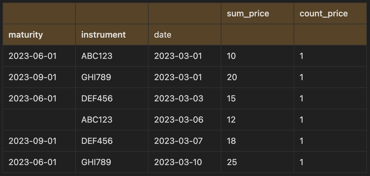
If we want to output some data with multi indexes, we can also make tweaks to swap the levels in the axis to achieve the desired format. For example, you could return to the original multi index dataframe above and swap the ordering of the columns in the index (swap date with maturity):

trades_df.groupby(['date', 'instrument', 'maturity']).agg(
    sum_price = ('price', 'sum'),
    count_price = ('date', 'count')
).swaplevel(0)

Or you could swap the axes, so that the columns now become the axis:

trades_df.groupby(['date', 'instrument', 'maturity']).agg(
    sum_price = ('price', 'sum'),
    count_price = ('date', 'count')
).swapaxes(0,1)

Melt & stack

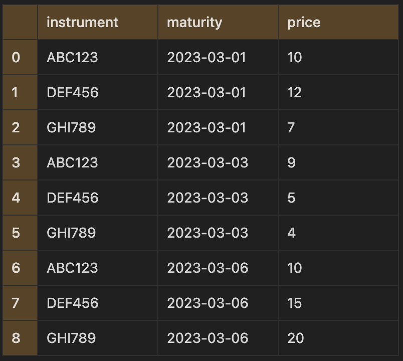
The methods melt and stack reshape data in the same way, with the difference that the melt method does not work when data is in the index, while stack does. For example, taking the following data, we can reshape it so that we have three columns instead: the instrument, maturity date and price:

df.melt(id_vars="instrument", value_vars=["2023-03-01", "2023-03-03", "2023-03-06"])

Here the id_vars parameter are the column names to remain the in vertical position and value_vars are the columns to reshape into a single column.

We can even rename the columns within the function and avoid listing out the columns we are melting by using:

df.melt(id_vars="instrument", var_name="maturity", value_name="price")

Here, all the columns not included in the id_vars parameter will be reshaped, so we can avoid having to list out all the columns.

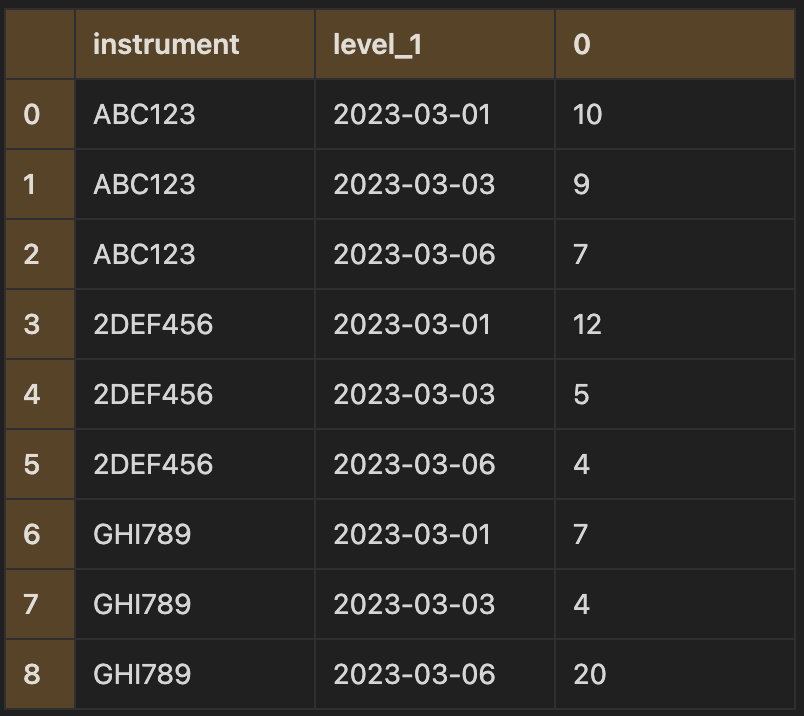
The stack method can produce almost the same output, but the reshaped column will instead be in the index. To replicate the transformation above, we will need to first set the index to the columns that will not be reshaped:

df_index = df.set_index("instrument")

Then we use the stack method to get the same output as melt:

df_index.stack()

instrument
ABC123 2023-03-01 10
2023-03-03 9
2023-03-06 7
2DEF456 2023-03-01 12
2023-03-03 5
2023-03-06 4
GHI789 2023-03-01 7
2023-03-03 4
2023-03-06 20
dtype: int64

This returns a series object with a multi index with two levels, so we’ll need to reset the index to get a single index dataframe:

df_index.stack().reset_index()

However, we’ll then need to rename the columns again, so the melt method would be a better option out of the two to avoid multi indexes and renaming columns.

Pivot & unstack

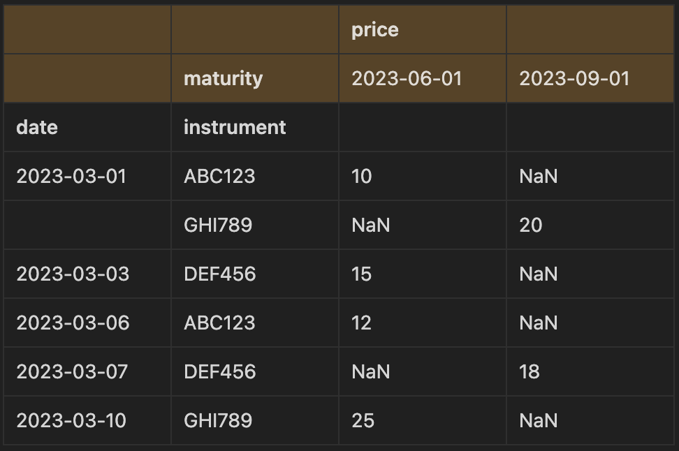
In Pandas, groupby and pivot_table produces the same data output but in a different shape. For example, taking the trade data, we can apply the pivot_table method as follows:

trades_df.pivot_table(index=["date", "instrument"], columns='maturity', values='price', aggfunc='sum')

Using the group by method as before, we would get:

trades_df.groupby(['date', 'instrument', 'maturity']).agg(
    price = ('price', 'sum')
)

In the pivot_table method, we pivot on the maturity date so that the unique values are now the column names. When doing data analysis, one might prefer to use the pivot table method to produce a more readable output and compare values across groups, whereas the group by method would be better suited for subsequent analysis and manipulation.

The unstack method is similar to the pivot_table method, except that it works with the values in the index. We need to first set the index to contain the columns that we would have assigned to the parameters index and columns in the pivot_table method, then apply the unstack method:

trades_df_index = trades_df.set_index(["date", "insturment", "maturity"]).unstack()

We now have a similar result as was produced with the pivot method, except that there is a multi index.

Modern Data Engineering